On “Defending Against Malicious Reorgs in Tezos Proof-of-Stake”

Note: We would like to acknowledge Bruno Blanchet (Inria) for his feedback. The interested reader can experiment with our code used in the analysis.

We are happy to note a new paper on Emmy⁺: “Defending Against Malicious Reorgs in Tezos Proof-of-Stake” by Michael Neuder, Daniel J. Moroz, Rithvik Rao, and David C. Parkes in the ACM Advances in Financial Technologies 2020 conference.

We are delighted that Tezos and Emmy⁺ are stimulating independent research activity, and we hope to see much more of this in the future.

The paper mainly studies the rate at which malicious forks can occur, developing on ideas put forward in our blog post on analyzing Emmy⁺. Where the paper’s analysis overlaps with our analysis, its conclusions agree with ours overall.

We also note a nice feature of the paper: a chain health metric (Section 5), which allows users to “identify potentially vulnerable chain states and take extra care with accepting large transactions”. This is close to our notion of accumulated/observed delay: the higher the accumulated delay, the less healthy is the chain and the more confirmations a user should wait for: see the “Forks started in the past” section part of our Emmy⁺ analysis.

We’d now like to discuss:

1. an alternative concrete choice of parameter values for Emmy⁺ considered in the paper, and

2. the methodology of our original analysis.

The concrete choice of parameters

The paper considers an alternative set of parameter values for Emmy⁺ (Subsection 4.3). For this choice, the rate of “forks starting now” is smaller when considering high attacker stake fractions (e.g. 0.4 or more).

The exploration of the parameter space is interesting, but we chose our parameter values as we did for quite practical reasons: we believe that in the real world, attackers will probably attack from a position of relatively smaller stake (less than 0.4, say), and for reasons discussed in detail below (“Comparing the two approaches”) we find the “forks started in the past” scenario more appropriate for defending Tezos against malicious forks.

The methodology

The paper’s approach is mostly simulation-based (Monte Carlo with importance sampling): exact probability calculations are given only for short fork lengths because the method used is enumeration based and thus it “quickly becomes computationally intractable” (Subsection 2.6 & Appendix A, B).

The data in our previous blog post was entirely generated by an efficient implementation of an exact method for computing probabilities. We describe it in the more technical part of the post below (“On the methodology”) where we show that calculating probabilities is, in fact, linear in fork length, and quadratic in the number of samples used to approximate the relevant probability distributions. More samples gives the analysis more precision, but we can still compute usefully precise probabilities for a large range of attacker stake fractions — even as high as 0.4-0.45, depending on the experiment.

Now, for the benefit of the more technically-minded reader, let’s take a closer look at the details:

On choosing the constants

Nomadic Labs’ approach

We recall that the parameters ie, dp, de were chosen while designing Emmy⁺. That is, they were chosen for the Babylon update. The reward policy has changed in Carthage to take into account various profitability criteria of selfish bakers, in particular criteria that take inflation into account.

The methodology used in our previous blog post was as follows:

• We tried to minimize both the feasibility of malicious forks, and of “block stealing”, that is, the feasibility of selfish baking. However, we did not take the profitability of selfish baking into account, the idea being that the reward policy can deal with this aspect. We believe that finding both the parameters ie, dp, de, and also the reward policy in a single step is too complicated: the search space is too big, and it is even harder to obtain an intuition on the dependencies between the parameters.

• We first observed that it is sufficient to search for appropriate values of ie and dp/de.

• We took the range of ie as [16, 30] (with a step of 2) and that of dp/de [1,20] and, for stake fractions from 0.2 to0.45 (with a step of 0.05), we computed the rate of malicious forks and the rate of block stealing.

• For malicious forks, we considered the “forks started in the past” scenario, assuming that a fork has started 5 blocks in the past and the observed delay during these 5 blocks was equivalent to 16 missing endorsements.

• Among these values for ie and dp/de, we chose ie = 24 and dp/de = 5 as, at a visual inspection of the plots, they seemed to be a good compromise for the two conflicting minimization problems: minimizing the feasibility of malicious forks and minimizing the feasibility of block stealing.

• We then chose dp = 40 as it seemed to be a good interval to reduce the waiting time between blocks (with respect to the previous value used in Emmy, namely 75), while also being large enough to allow blocks and operations to be timely delivered.

The paper’s approach

The paper proposes an objective function (in Section 4.2, equation (14)) which weighs both the rate of malicious forks, and of selfish baking, for two given forks length, namely 20 for malicious forks and 3 for selfish baking. One would then look for parameter values that minimize this objective function.

The paper sets parameter values of ie=15, dp=8, and de=5. For an attacker stake fraction of 0.4 these values give a weighted probability, as given by the objective function, that is 2.5 times smaller (so better) than the current parameter values for Emmy⁺, namely, ie=24, dp=40, de=8.

Comparing the two approaches

First, the paper argues about the optimality of the new parameters in a quite particular setting: for high attacker stake fractions, and for specific and somewhat arbitrary forks lengths. However, these choices represent only a few points in a much larger space of possible combinations. It is unclear whether one would reach the same conclusion when looking at the whole space.

Second, the paper considers the “forks starting now” scenario and not the “forks started in the past” scenario, which is the one a user is ultimately interested in: ideally, a user would not blindly wait for a number of confirmations (as provided by the “forks starting now” scenario), instead she would look at the health of the chain since the time her transaction was included and would take this information into account (as in the “forks started in the past” scenario).

Note that using “forks started in the past” scenario means that we compare a rather healthy chain (the case that is most often observed) to a chain made by the adversary. In contrast, if we look at “forks starting now” scenario, the honest chain is typically less healthy, since the adversary does not provide endorsements and does not bake on the honest chain. In other words, when looking at the “forks started in the past” scenario, we would optimize for the desired case, while when looking at “forks starting now” scenario, we would optimize for the worst case. So both approaches have their strengths.

Third, we would be cautious about choosing a small dp value, because this intuitively means that if the block at priority 0 is missing, then the bakers at the following priorities (say 1, 2, 3) have little time to see each other’s blocks, so we might get that half of the network is on the block at priority 1 and half on the block at priority 2 (assuming that all the endorsements have already arrived). However, one could still achieve the same proposed dp/de ratio of 8/5 with higher dp values, e.g. dp=40 and de=25.

In what follows we revisit and improve parts of our previous analysis to understand how the newly proposed parameters compare with the ones currently used by Emmy⁺. For completeness, we provide the code used for our experiments.

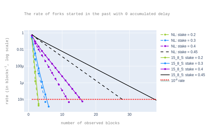
For the sake of comparison, we replot forks started now/in the past with ie=15 and dp/de=8/5.

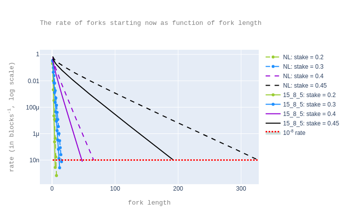
So for “forks starting now”, the choice proposed in the paper is better.

However, the choice (ie,dp/de)=(24,5) is slightly better for “forks started in the past” scenario for observed delay 0.

In an attempt to be more systematic, inspired by the paper, we plotted a few additional contour maps.

On the methodology

The main point of this section is to show that the complexity of our approach is linear in the length of the fork. Said otherwise, an analytical approach does not need to be exponential in the length of the fork, as suggested in the paper.

Our approach is to compute the probability distribution of the time difference between the attacker’s chain and the honest chain, while assuming both chains have equal length. By the “time of a chain” we mean the timestamp of the head of the chain. Note that the attacker is able to produce a fork if and only if this difference is smaller than 0.

The probability distribution is computed on a bounded sample space. Namely, we fix lower and upper bounds on the timestamp difference. Concretely, we only computed the probabilities that the difference is in the interval [-m'/2, m'/2], for some constant m'. Note that the higher m', the higher the precision of the analysis.

As showed in the previous blog post, it is the ratio dp/de that matters in this analysis. For convenience, we have assumed that dp is a multiple of de. Therefore we have that any possible timestamp difference is a multiple of de. This means that we can represent the probability distribution by an array of size m where m'=m/de and where an index i corresponds to the difference (i-m/2)*de.

In our experiments, m was usually 2001. This is sufficient, in that we do not lose too much precision: we checked that the sum of all probabilities in the bounded sample space is still 1 and not smaller (or at least not significantly smaller).

We illustrate in more detail how the probability distribution is computed for the “forks starting now” case. The other cases are similar.

The main idea is to compute the probability distribution inductively: given the probability distribution for forks of length n, compute the probability distribution for forks of length n+1. Then, at each iteration we check whether we reached a fork length for which the probability that the attacker’s chain is faster than the honest chain is smaller than the security parameter. The pseudo-code of the main procedure is given below.

one_level_pd := init(first_level=False)
pd := init(first_level=True)
win_p := 0
fork_len := 1
while win_p > 1e-8:
    pd := sum_pds(pd, one_level_pd)
    win_p := pd[:m/2].sum()
    fork_len++
return fork_len

The init procedure computes the probability distribution of the difference between the delay of the attacker’s block and of the honest block at some arbitrary level. Recall that if the level is that of the first block of the fork, then the attacker can also include the endorsements of the honest parties, while otherwise it can only include its own endorsements. This distinction is captured with the first_level argument.

The init procedure iterates through the m possible differences and the 33 possible number of endorsements the attacker might have. For each combination we determine the priorities the attacker and the honest parties should have in order to obtain the corresponding difference. Based on this information, we compute the probability to obtain the given difference.

The sum_dps procedure basically computes the convolution of two probability distributions. In our case, sum_pds computes the probability distribution of the difference between chains of length n+1 as the convolution of the probability distribution between chains of length n and the probability distribution of the difference between chains of length 1. Concretely, sum_pds goes through all pairs (i,j) of indexes in pd and respectively one_block_pd, such that the differences d_k and d_1 corresponding to indexes i and j add up to a difference d_{k+1} = d_k + d_1 in the [-m'/2, m'/2] interval. In that case the new probability associated with the difference d_{k+1} is updated to p_{k+1} := p_{k+1} + p_k * p_1, where p_k is the probability associated with d_k in pd and p_1 is the probability associated with d_1 in one_level_pd. (p_{k+1} is initially set to 0.)

The main procedure is then a simple while loop in which at each iteration we compute the probability that the attacker’s chain is faster than the honest chain. This condition is equivalent to saying that the difference between the two chains is negative. This is why the corresponding probability is obtain as the sum of the probabilities in the first half of the pd array.

From the explanations above, it is easy to see that the time complexity of a call to init is O(m) and the time complexity of a call to sum_pds is O(m^2). We conclude that the complexity of this approach is linear in the length of the fork and quadratic in m.

A visual explanation

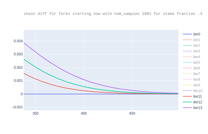
We plot the arrays pd for f=.3 and m=1001. We intentionally consider a rather small value of m because it is small enough that we get errors bigger than 1e-9, where by “error” we mean the difference between 1 and the sum of all probabilities in pd.

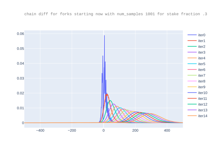
For a value x0 on the x-axis, the corresponding point y0 in the curve for a given iteration represents that the probability that the difference between the attacker chain and the honest chain is x0*de. Recall that the attacker chain is faster (so attacker’s fork “wins”) if and only if this difference is smaller than 0. Therefore, for a given iteration i the area under the curve iteri at left of 0 approximates the probability that an attacker wins for any difference with a fork of length i+1, while the total area should be 1. We note however that since the curves go a bit more to the right at each iteration (as the expected time difference between the chains increases) computing the total sum up to m/2 loses data (the truncated part of the shifted curves). To see this more clearly, we zoom in.

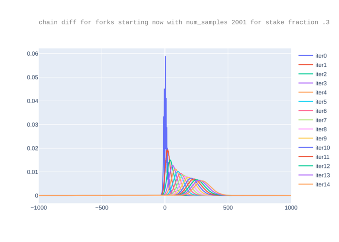
For m=2001, we no longer get an error thus this sample size is sufficiently large to not lose information.

Though for m=1001 the results are imprecise with respect to the total sum, the resulting probabilities are the same as for m=2001. This is because the truncation only affects visibly the right-hand side while the probability that the attacker wins is on the left-hand side of 0: the lost data on the right-hand side does not have a visible impact. Still, for safety we updated the code so that if the sum is not close to 1, an error is raised suggesting the user to use a larger m.

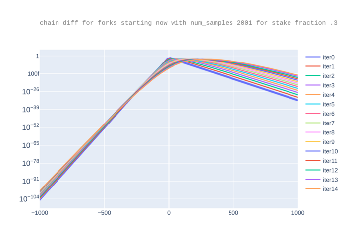
For completeness, we add a version of the previous plot, where the y-axis is in log scale.

Appendix

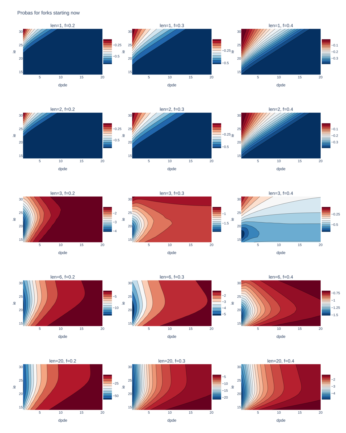
Instead of heatmaps, we plot contour maps, in log scale, as we find they suit our purpose better in that we can see clearly the delimitations between different security thresholds (represented by different coloured regions). As the security threshold we considered so far is \(10^{-8}\), the region of interest in each plot is the one with the colour corresponding to -8 in the colour bar.

In the plots below, the z-axis is the probabilities for forks starting now, resp. in the past.

For forks starting now, we consider the fork lengths 1, 2, 3, and 6 and 20 and exhaustively explore the following ranges for ie and dpde: ie ranges from 14 to 32 and dpde ranges from 1 to 20.

The plots suggest that smaller dpde values are better.

This is not necessarily the case for forks started in the past. We consider stake fractions .2, resp. .3 and we vary the accumulated delay for 3 seen blocks for .2, resp. 5 and 10 seen blocks for .3. (We recall that 3, resp. 5 were the expected confirmation numbers for .2, resp. .3 when the accumulated delay is 0). Precisely, what we denote by odr in the plots represents the accumulated (or observed) delay divided by de and odr ranges over {0, 16, 32, 64, 128}.

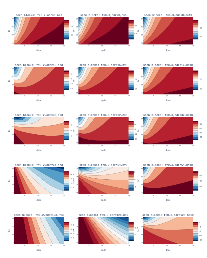
The above plots suggest that higher ie values are better. Moreover, we find that it is more important to choose higher ie values despite the observation that smaller ie values are “better” when considering forks starting now. This is because for forks started in the past, a small ie may cause high fork probabilities. For instance: if the attacker stake fraction is .2, the number of seen blocks is 3, odr is 32, and dpde is around 5, then the probability of a fork can go up to \(10^{-2}\) for small ie values such as 15. In contrast, for the same setup but with high ie values such as 30, the probability of a fork remains smaller than our security threshold of \(10^{-8}\).

And finally: we had not previously considered smaller ie values (as this was against the “raison d’être” of Emmy). We checked this with some experiments as illustrated in the plots below, in which ie ranges from 0 to 14. These plots demonstrate that for such small ie values, the fork probabilities are high (compared to the above plots for forks starting now), and that higher ie are better.